The Mandelbrot Set: An Answer Key and Discussion Post
This article is a response blog post to the following 3blue1brown video about Holomorphic Dynamics (one of a large series of interesting and informative math videos.) This blog post is my attempt to write an answer key to some of the explicit exercises that Grant Sanderson puts out in his video essay as well as talk about and explore some of the finer points he alludes to in Complex Analysis and Holomorphic Dynamics.
Exercise 1: When are Mandelbrot fixed points stable?

1a: Find the fixed points of $f(z)=z^2+c$.
We only need to solve the equation $f(z) = z$ or $z^2+c=z$ which means solving the quadratic $z^2-z+c=0$. This can easily be seen to be \[ z_0^\pm = \frac{-(-1)\pm \sqrt{(-1)^2-4*1*c}}{2*(1)} = \frac{1}{2} (1 \pm \sqrt{1-4c}) \]
I should probably make note of the fact that we are using the symbol $\pm$ to denote both the positive and the negative square root of the complex number $(1-4c)$. If this is your first time dealing with the complex square root function it may be of interest to verify that there will always be two roots of any complex number and that one is the negative of the other. In the special case of zero this corresponds to a double root at the point zero. In our case, this corresponds to when $1-4c=0$ or $c=\frac{1}{4}$. Here our original fixed point equation becomes $z^2-z+\frac{1}{4} = (z-\frac{1}{2})^2$ and both the fixed points of our iterative function f are located at $z_0=\frac{1}{2}$.
1b: Determine when at least one fixed point is attracting.
We now need to find when these fixed points that we have found are attracting meaning they satisfy $|f'(z_0)|<1$. As mentioned in the video, this will correspond to our point being sucked in towards this fixed value instead of pushed away, resulting in the stable dynamics we expect from the black parts of the Mandelbrot set. The derivative of f can easily be calculated to be f'(z)=2z so our attracting equation requires that $|2 \cdot z_0^\pm|<1$ for either the positive or the negative root. This means we need $|1\pm \sqrt{1-4c}|<1$ for either the positive or negative case.
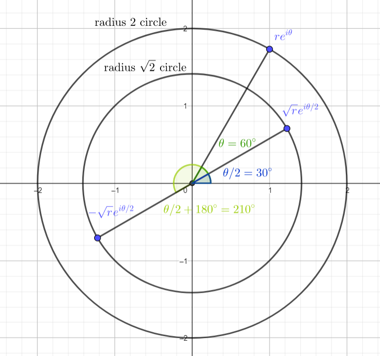
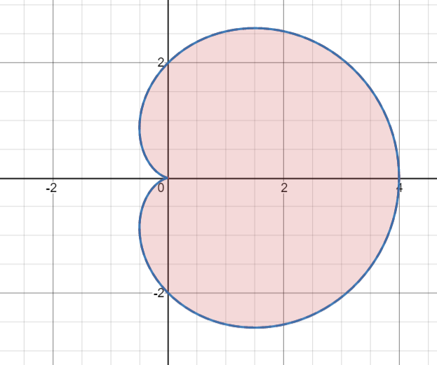
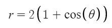
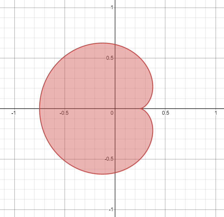
Let us take the complex number $\sqrt{1-4c}$ to be represented by $a+bi$. If we say that $1-4c$ is the complex number represented by $re^{i\theta}$ then it quickly follows that $a=\pm\sqrt{r}\cdot cos(\theta/2)$ and $b=\pm\sqrt{r}\cdot sin(\theta/2)$ from our understanding of the complex square root. Our original requirement becomes: \[|1+a|^2+|b|^2<1\] or \[(1\pm\sqrt{r}\cdot cos(\theta/2))^2+(\pm\sqrt{r}\cdot sin(\theta/2))^2 = \] \[1 \pm 2\sqrt{r}\cdot cos(\theta/2) + r\cdot cos(\theta/2)^2 + r\cdot sin(\theta/2)^2 <1\] or \[ \pm 2\sqrt{r}\cdot cos(\theta/2) + r\cdot (cos(\theta/2)^2 + sin(\theta/2)^2) <0 \] giving \[ r < \mp 2\sqrt{r}\cdot cos(\theta/2) \] giving \[ \sqrt{r} < \mp 2\cdot cos(\theta/2) \] squaring then yields: \[ {r} < (\mp 2\cdot cos(\theta/2))^2 = 4(cos(\theta/2))^2 = 4( (1+cos(2*\theta/2))/2) = 2(1+cos(\theta)) \] This shape $r=2(1+cos(\theta))$ corresponds exactly to the cardioid shape we want to find. Hence by a simple shift of $c=\frac{1}{4}(-re^{i\theta}+1)$ gives us the exact location of the shape in the Mandelbrot set.
1c: Show that this set of c values forms the distinctive cardioid shape.
Now that we have gotten our distinctive cardioid shape to show up in our equations, let's work just a little bit harder to show the exact cardioid which shows up in our Mandelbrot formulation. Bringing ourselves back to the equation: \[ \sqrt{r} < \mp 2\cdot cos(\theta/2) \] and viewing the plots of the two functions on the RHS of the above equation:
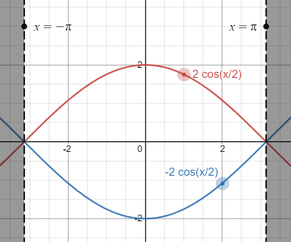
We can see that our $\sqrt{r}$ value on the LHS of the equation is what we are assuming to be the positive square root. Hence, when we see in our image that $-2 cos(\theta/2)$ function is always below zero for the values of $\theta \in [-\pi,\pi]$, we know that this will never correspond to valid values for $\sqrt{r}$. If we follow our calculations to the beginning, we will see that this corresponds to the positive root $z_0^+$ being unstable/ repelling and the negative root $z_0^-$ being stable/ attracting. As a quick example, let's take $c=0$ giving roots $z_0^\pm = \frac{1}{2} (1 \pm \sqrt{1}) = 1,0$. This corresponds to the iterative map $z\to z^2$ which we know that $1$ is indeed a fixed point for, but every number that is very close but not equal to one will either shrink to zero or shoot off to infinity (or technically spin around the unit circle.) This corresponds to $1$ being an unstable fixed point. Zero, however, is a stable fixed point and every number that is small enough (in fact smaller that norm one) will shrink to zero after repeated squaring. For general $c$, the same intuition holds that the positive root adds a positive number to $\frac{1}{2}$ making it even larger when positive, which pushes the fixed point away from the stability near zero and has more similar behavior to $1$ under repeated squaring.
Anyways, let's compute our Mandelbrot set cardioid now that we know which root to be looking at and don't have to worry about any boundary conditions. As we already claimed, the shape $r=2(1+cos(\theta))$ corresponds exactly to the cardioid we want to find. We only need to shift our $(1-4c) = re^{i\theta}$ to solve for the value of $c$. The simple shift $c=\frac{1}{4}-\frac{1}{4}re^{i\theta}$ gives us the location of the shape in the actual Mandelbrot set. Visually, we can see this corresponds to flipping our cardioid horizontally, dividing it by a factor of 4, and shifting it over by $-\frac{1}{4}$.
Exercise 2: Attractive cycles in Newton's method
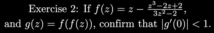

We can use the fact that $P(z) = z^3 -2z +2$ and $P'(z) = 3z^2-2$ to explicitly calcualte $f$ and $f'$ as \[ f(z) = z - \frac{z^3 -2z +2}{3z^2-2} = \frac{z(3z^2-2) - (z^3 -2z +2)}{3z^2-2} = \frac{2z^3-2}{3z^2-2} \] \[ f'(z) = \frac{(3z^2-2)*(6z^2)-(2z^3-2)(6z)}{(3z^2-2)^2} = \frac{6z( 3z^3-2z-2z^3+2)}{(3z^2-2)^2} = \frac{6z(z^3-2z+2)}{(3z^2-2)^2}\] First, let's confirm that there is indeed a cycle at $0$. Let's plug in zero to our function $f$: $f(0) = \frac{2\cdot 0^3-2}{3\cdot 0^2-2} = \frac{-2}{-2} = 1$. So then let us plug in $1$ to our function $f$: $f(1) = \frac{2\cdot 1^3-2}{3\cdot 1^2-2} = \frac{2-2}{3-2} = 0$. Now if we define $g(z)=f(f(z))$ we can see that $g(0)=0$ since $0$ is part of a 2-cycle. We now want to calculate $g'(0)$ to show that it is indeed an attracting cycle. We know by the chain rule that $g'(z) = f'(f(z)) \cdot f'(z)$ so then it follows that $g'(0) = f'(1)\cdot f'(0)$. \[ f'(0) = \frac{6\cdot 0\cdot (0^3-2\cdot 0+2)}{(3 \cdot 0^2-2)^2} = \frac{0}{4} = 0\] \[ f'(1) = \frac{6\cdot 1\cdot (1^3-2\cdot 1+2)}{(3 \cdot 1^2-2)^2} = \frac{6(1-2+2)}{1} = 6\] So it follows that $g'(0)=0$ and that $|g'(0)|<1$, in fact since it is equal to zero this is indeed a super attracting 2-cycle.
Exercise 3: Attractive cycles in Newton's for cubic polynomials?


[Fatou's 1919 Theorem] One of the solutions of $f'(z)=0$ must fall into an attracting cycle if there exist any attracting cycles. Use this theorem to show verify the fact that if there is an attracting cycle then $z_0 := (r_1 + r_2 + r_3)/3$ will fall into it.
proof: Recall that $f'(z) = \frac{P(z) P''(z)}{(P'(z))^2}$ so then if we have that $f'=0$ it follows either $P=0$ which means we are looking at a root which we already know is an attracting fixed point or that $P''=0$. Hence, we only need to focus on the case where $P''(z)=0$ to look for our attracting cycles. We can then use the fact that a simple cubic $P(z)$ can be rewritten as $P(z) = c(z-r_1)(z-r_2)(z-r_3)$ for some constant c. By utilizing the chain rule multiple times we get that: \[ P'(z) = c\cdot [(z-r_1)(z-r_2)+ (z-r_1)(z-r_3) + (z-r_2)(z-r_3)] \] \[ P''(z) = c\cdot [(z-r_1) + (z-r_2) + z-r_3)] = c(3z - r_1 -r_2 -r_3)\] So then if $P''(z) = 0$, then $(3z - r_1 -r_2 -r_3)=0$ or $z = (r_1 + r_2 + r_3)/3 =z_0$. Hence, we need to only check this one value $z_0$ where $P''(z)=0$ to search for an attracting cycle, exactly as claimed in the video.
Further Discussion: Computing the Mandelbrot Set
Degree Two Cycles
Continuing to compute the attracting cycles of the Mandelbrot set we can start with the degree two cycles. This creates a quartic polynomial to solve which we can still do in closed form but will have ridiculously more complicated expression than the quadratic solution we looked at earlier. Fortunately, we can reduce this quartic expression by dividing by the fixed points we have already found $\frac{f^2(z)-z}{f(z)-z}$ where $f(z)=z^2+c$ is the Mandelbrot $f$, since we know they will also satisfy this polynomial equation. Our reduction leaves us with a quadratic polynomial again which we can easily solve for with the quadratic formula: $z^2+z+(c+1)=0$. \[ z_1^\pm=\frac{1}{2}(-1 \pm \sqrt{1-4(c+1)})\] We should be able to confirm that these two roots cycle with each other each corresponding to the same 2-cycle: \[f(z_1^+) = (\frac{1}{2}(-1 + \sqrt{1-4(c+1)}))^2 + c = \frac{1}{4}(1 - 2\sqrt{1-4(c+1)} + 1-4(c+1)) + c\] \[ = \frac{1}{2}(1-2c-2 - \sqrt{1-4(c+1)} +2c) = \frac{1}{2}(-1 - \sqrt{1-4(c+1)}) = z_1^- \] \[f(z_1^-) = (\frac{1}{2}(-1 - \sqrt{1-4(c+1)}))^2 + c = \frac{1}{4}(1 + 2\sqrt{1-4(c+1)} + 1-4(c+1)) + c\] \[ = \frac{1}{2}(1-2c-2 + \sqrt{1-4(c+1)} +2c) = \frac{1}{2}(-1 + \sqrt{1-4(c+1)}) = z_1^+ \] We now want to check when this is an attracting cycle. This again requires checking when the absolute value of the derivative is smaller than one, but now we need that the derivative of the second iterate $f(f(z))$ to be smaller than one, not just the derivative of either of the cycle points. One could imagine that one of the points pulls in nearby points at a rate of 1/2, but this doesn't matter if the other point in the cycle pushes points away at a rate of 10. This would still be a repelling cycle. So, now we need that $f'(z_1^+)\cdot f'(z_1^-) = |2*z_1^+|*|2*z_1^-|<1$ or that $|-1+\sqrt{1-4(c+1)}|*|-1-\sqrt{1-4(c+1)}|<1$. If we similarly prescribe that $1-4(c+1) = re^{i\theta}$ and that the square root $\sqrt{1-4(c+1)}$ is $a+bi$, then the norm together is: \[ ((-1+a)^2+(b^2))*((-1-a)^2+((-b)^2))=(1-2a+a^2+b^2)*(1+2a+a^2+b^2)=1-4a^2+(a^2+b^2)^2+2(a^2+b^2)<1\]. This becomes: \[ 1 -4[r/2(1+cos(\theta))]+r^2+2r<1\] or \[-2(1+cos(\theta)-1)+r<0\] or \[r<2cos(\theta)\]. We know from polar coordinates that this corresonds to a circle of radius 1 centered at (1,0). Finally, we can shift over our circle with $c=-\frac{1}{4}(re^{i\theta})-\frac{3}{4}$ which gives us a circle of radius one fourth centered at -1.
Conveniently, this circle exactly touches the cardioid we just calculated at the point $-\frac{3}{4}$ so it looks like we are on the right track. At this point, I think another pertinent question is why the existence of any attracting cycle corresponds to an exact region of the Mandelbrot set. A priori, we have no reason to expect that the existence of an attracting cycle will necessarily mean that the trajectory starting at zero will eventually fall into it. This is an important last step to proving that the regions we are calculating actually correspond to the Mandelbrot set. We push this question to the later section filling the gaps (in Complex Analysis) of the original video and this blog post.
Calculating Higher Degree Cycles
Continuing on in our journey to calculate the Mandelbrot set, we next check the third degree cycles which are the solution to the $2^3=8$ degree polynomial except for the (2) fixed points: \[ \frac{f^3(z)-z}{f(z)-z} = z^6 + z^5 + (3c+1)z^4 + (2c+1)z^3 + (3c^2+3c+1)z^2 + (c^2+2c+1)z + (c^3+2c+c+1) \] Unfortunately, this leaves us with a sixth degree polynomial that nobody wants to solve. We could try solving for these roots numerically (using Newton's method of course :^) ); however, we are currently trying to solve for an equation in terms of $c$ which is an unknown variable, so we would need to apply a numerical solver like Newton's method at every possible value of $c$.
This left me stuck for a while, but in trying to calculate the attractiveness of a 3-cycle: $|f'(z^{(1)})\cdot f'(z^{(2)})\cdot f'(z^{(3)})|<1$, I realized that while I may not be able to calculate the cycles exactly, I am able to find which $c$ values will have a superattracting orbit. This will correspond to when the initial starting point of the Mandelbrot iteration (zero) is also in the cycle, because $f'(z)=2z$ is zero only at $z=0$.
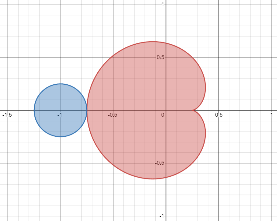
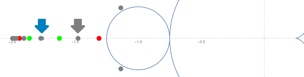
This means that the roots of our sixth degree polynomial $\frac{f^3-z}{f^1-z}$ has $z=0$ as a root. But we also know from basic theory of algebra that the product of all the roots of a polynomial will equal the constant term. For zero to be a root means the product of all the roots will itself too be zero, and hence we only need to look at the solutions to the constant coefficient $(c^3+2c+c+1)$ of the rather large sixth-degree polynomial. Notably, this only a third-degree polynomial for which we can solve explicitly and the roots are approximately $-1.755$, $-0.12256+0.74486i$, and $-0.12256-0.74486i$. Plotting these alongside what we have so far gives us:
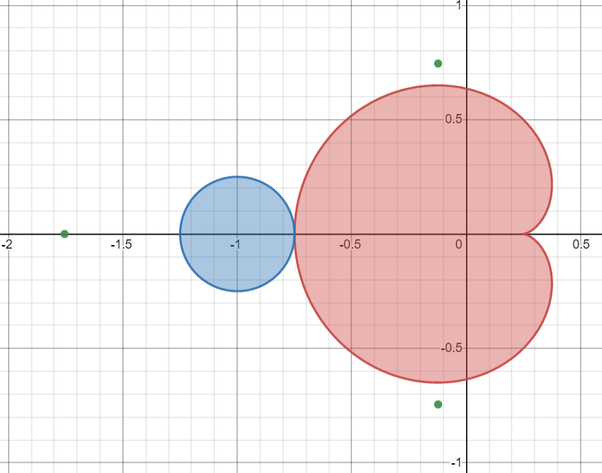
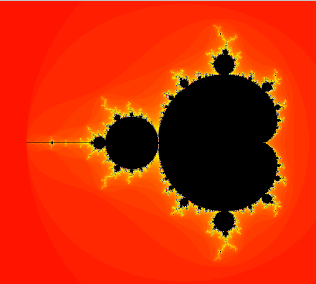
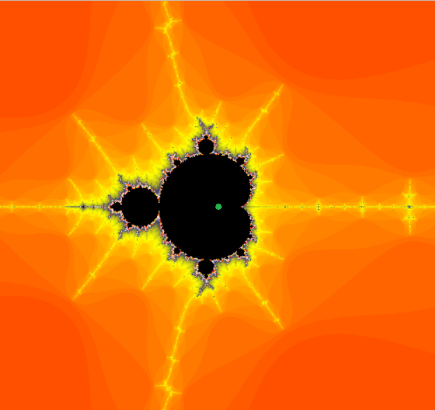
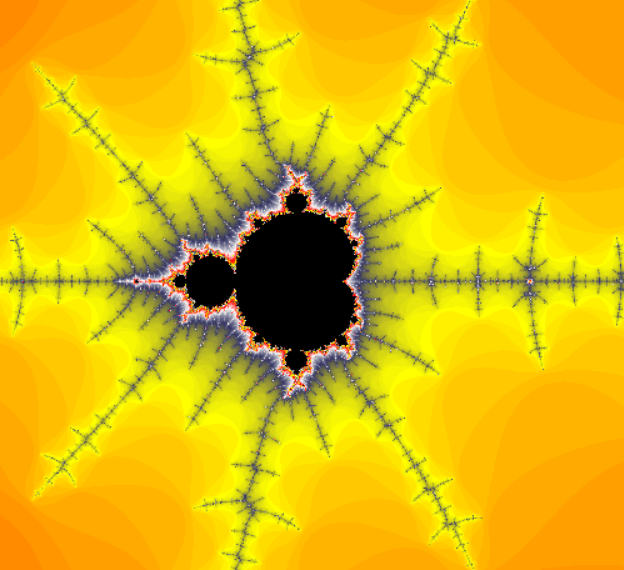
If we look at a graphic of the Mandelbrot set we can indeed see that this corresponds to black attractive regions of the Mandelbrot set. Interestingly, while the two complex values correspond to the 1/3 bulb and the 2/3 bulb of the Mandelbrot set, the negative real location on the far left corresponds to the main cardioid of the first Minibrot of the Mandelbrot set. Zooming in to this location we can see the first (and largest) Minibrot:

Now let's talk a little bit more about how many cycles of order $n$ we expect. We know that we can solve the degree $2^n$ polynomial, but we also can get rid of lower order solutions like we have been getting rid of the fixed points by dividing the polynomial by $f(z)-z$. Let's denote $F_n(z) = f^n(z) - z$ the $n$-th degree fixed point equation. Let us additionally take $G_n(z)$ to be $F_n(z)$ after we divide by all of the redundancies corresponding to lower-order cycles. This means: \[ G_1(z) = F_1(z) = z^2 - z + c \] \[ G_2(z) = \frac{F_2(z)}{F_1(z)} = z^2 + z + (c+1) \] \[ G_3(z) = \frac{F_3(z)}{F_1(z)} = z^6 + z^5 + (3c+1)z^4 + (2c+1)z^3 + (3c^2+3c+1)z^2 + (c^2+2c+1)z + (c^3+2c+c+1) \] \[ G_4(z) = \frac{F_4(z)}{F_2(z)} = \frac{F_4(z)}{G_1(z)\cdot G_2(z)} = z^{12} + 6c z^{10} + z^9+ (3 c + 15 c^2) z^8 + 4 c z^7 + (1 + 12 c^2 + 20 c^3) z^6 + (2 c + 6 c^2) z^5\] \[ + (4 c + 3 c^2 + 18 c^3 + 15 c^4) z^4 + (1 + 4 c^2 + 4 c^3) z^3 + (c + 5 c^2 + 6 c^3 + 12 c^4 + 6 c^5) z^2 + (2 c + c^2 + 2 c^3 + c^4) z + (1 + 2 c^2 + 3 c^3 + 3 c^4 + 3 c^5 + c^6) \] In general, we can see that: \[ G_n(z) = F_n(z) \cdot \left[\Pi_{k \hspace{0.25em}\text{divides}\hspace{0.25em} n} (G_k(z)) \right]^{-1} \] If we take $d_n$ to represent the degree of $G_n(z)$ we can see that: \[ \sum_{k \hspace{0.25em}\text{divides}\hspace{0.25em} n \hspace{0.25em}\text{(including n)}} d_k = 2^n \] Then we can use some number theory to show that when we take the prime factorization representation of $n = p_1^{a_1} \cdot \dots \cdot p_l^{a_l}$ we can solve for $d_n$ as: \[ \large d_n = \sum_{\alpha_1 = 0}^1 \dots \sum_{\alpha_l = 0}^1 (-1)^{\sum_{i=1}^l \alpha_i}\cdot 2^{p_1^{a_1-\alpha_1} \cdot\dots\cdot p_l^{a_l-\alpha_l}} \]
This formula is probably most easily verified by induction on $a$ and $l$. I don't believe this arithmetic function can be further reduced, but it possible there is a simpler formulation. This function is closely related to Euler's totient function $\varphi(n)$ which counts the number of integers coprime to $n$. We can see that $\{d_n\} = 2,2,6,12,30,54,\dots$ which is available at https://oeis.org/A027375. It follows that the number of distinct cycles is ${d_n}/{n}$ since there are n different points in an n-cycle. We can see that $\{d_n/n\} = 2,1,2,3,6,9,18,\dots$ which is available at https://oeis.org/A001037.
Finding Higher Degree Basins
Although I personally was not able to figure out how to find the basins of attraction for the 3-cycles of the Mandelbrot set, as with most things, someone has already done it! At this website https://commons.wikimedia.org/wiki/File:Mandelbrot_Components.svg, they reference the method of "P-form boundary equations" to solve analytically for the 3-cycle. They then continue for the higher-order boundaries by using numerical approximations to plot the boundary regions.

We instead explore using the super-attractive cycle points to find the centers of our basins of attraction. This can done relatively easily by just numerically solving the $0$-th coefficient as we did before for the 3-cycle case: \[ G_4(z) [z^0] = \frac{F_4(z)}{F_2(z)} [z^0] = 1 + 2 c^2 + 3 c^3 + 3 c^4 + 3 c^5 + c^6 \] \[ G_5(z) [z^0] = \frac{F_5(z)}{F_1(z)} [z^0] = 1 + c + 2 c^2 + 5 c^3 + 14 c^4 + 26 c^5 + 44 c^6 + 69 c^7 + 94 c^8 + 114 c^9 + 116 c^{10} + 94 c^{11} + 60 c^{12} + 28 c^{13} + 8 c^{14} + c^{15}\] \[ G_6(z) [z^0] = \frac{F_6(z) F_1(z)}{F_2(z) F_3(z)} [z^0] = 1 - c + c^2 + 3 c^3 + 7 c^4 + 17 c^5 + 35 c^6 + 76 c^7 + 155 c^8 + 298 c^9 + 536 c^{10} + 927 c^{11} + 1525 c^{12} + 2331 c^{13} + 3310 c^{14} \]\[\hspace{6.em} + 4346 c^{15} + 5258 c^{16} + 5843 c^{17} + 5892 c^{18} + 5313 c^{19} + 4219 c^{20} + 2892 c^{21} + 1672 c^{22} + 792 c^{23} + 293 c^{24} + 78 c^{25} + 13 c^{26} + c^{27} \] \[ G_7(z) [z^0] = \frac{F_7(z)}{F_1(z)} [z^0] = 1 + c + 2 c^2 + \dots + 32 c^{62} + c^{63}\]


Maybe more importantly than the number of cycles which exist of each degree is the number of basins we get from these cycles. It seems very much like every super-attractive cycle we find corresponds exactly to one basin of attraction. Unfortunately, I am unable to prove that fact, but the number of basins follows $1,1,3,6,15,27,63, \dots$ which indeed follows the sequence https://oeis.org/A000740 which claims that it is the "number of components of the Mandelbrot set corresponding to an attractive n-cycle". Hence, the fact that is left unproven is that our method of finding super-attractive cycles via the constant coefficient of the fixed point polynomial will always have the same degree as this number of attractive basins. (Although it seems extremely likely.)
Let's do a little more exploration with the basins we have found at the tendril coming off of the $\frac{1}{3}$ ball from the main cardioid.

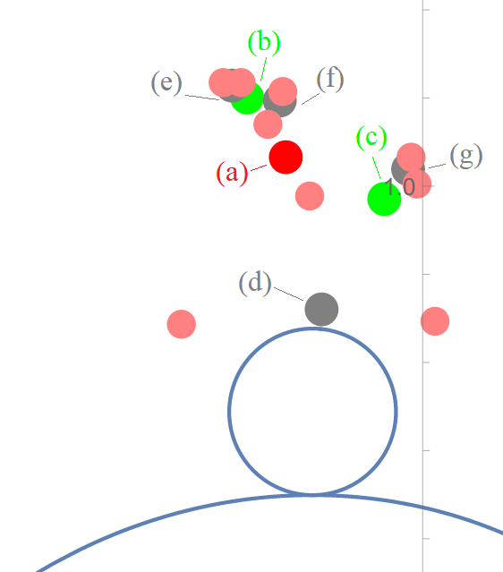
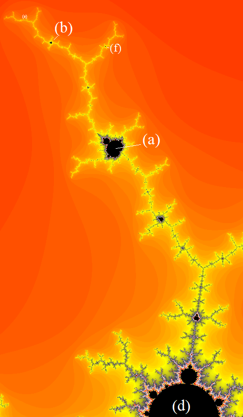
(a)
 (b)
(b) 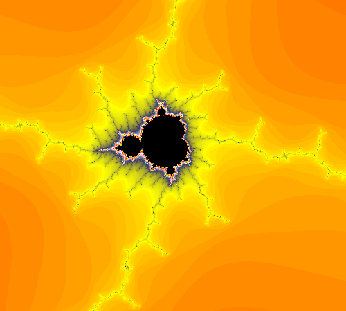 (c)
(c) 
(d)
 (e)
(e) 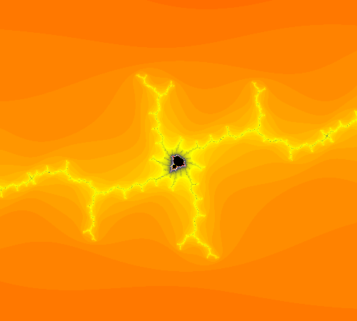
(f)
 (g)
(g) 
One More Cool Thing (Logistic Map)
Let us take a look at one more interesting part of the Mandelbrot set. The segment which intersects the real line is called the "Mandelbrot Needle". As we can see from our above calculations to find the basins, we can see that a whole host of the zeroes/ basins on the real line in the interval (-2,-1.25). In addition to the $1,2,4,8,\dots$ bulbs which attach on the left starting at the main cardioid and going to the left and shrinking in size. This corresponds to repeated period doublings as we go further and further to the left.
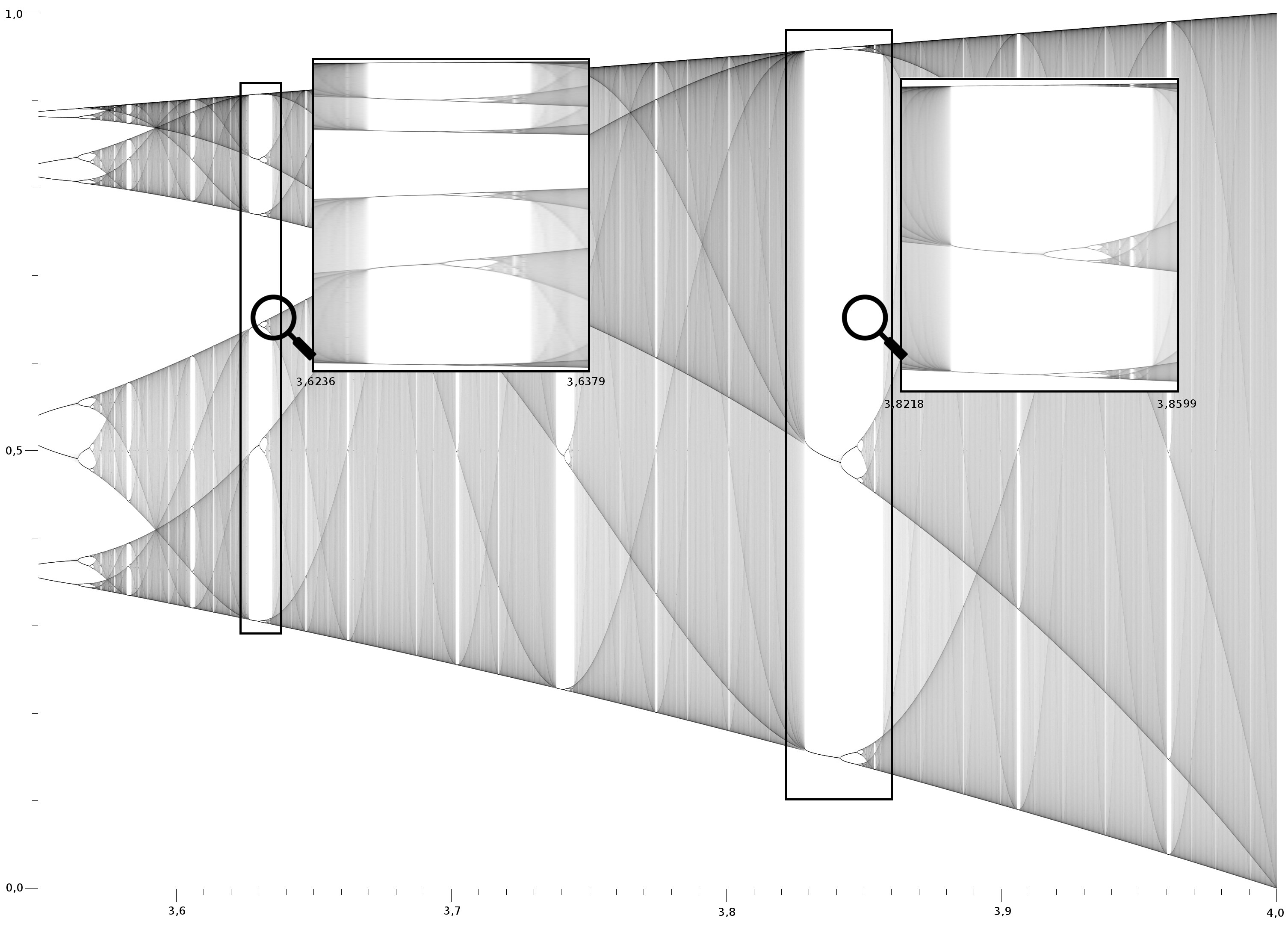
Here in the real line there is an extremely interesting connection with the logistic map and the bifurcation diagram. The logistic map studies something like the population of rabbits over time. Let's call the population at time $n$ to be $x_n\in(0,1)$ where we have rescaled so that $x$ is between zero and one (corresponding to the natural carrying capacity of the environment.) The logistic map takes the perspective that the population increases by reproduction when $x_n$ is large, but decreases by starvation when $x_n$ is too large (close to 1.) Consequently, the population at the next time step is $x_{n+1} = r x_n (1-x_n)$ where $r$ is some rate parameter for the logistic equation. The classical result from this logistic map is that as we vary $r$ to be larger and larger, we change from stability (1-cycle) where the population approaches a stable equilibrium population. To seasonality (2-cycle) where each year we go back and forth between a larger population size and a smaller population size. Continuing on, we get 4-cycles, 8-cycles, etc. Eventually, this procedure descends into chaos for high enough values of $r$. The bifurcation diagram showing the stable values for different $r$'s is plotted in high resolution below:

If you have not seen this diagram before it is interesting in its own right, but other resources will do a better job of explaining it than I am doing here. Interestingly, for our context of the Mandelbrot set, we will look at the transformation $u_n = r(x_n-\frac{1}{2})$ and $R=\frac{r(r-2)}{4}$. We can see that $x_n = \frac{u_n}{r} + \frac{1}{2}$ and that our iteration equation becomes: \[ (\frac{u_{n+1}}{r} + \frac{1}{2}) = r\cdot(\frac{u_n}{r} + \frac{1}{2})\cdot(1-(\frac{u_n}{r} + \frac{1}{2})) \] \[ u_{n+1} +\frac{r}{2} = (u_n + \frac{r}{2})\cdot (-u_n+\frac{r}{2}) \] \[ u_{n+1} = -u_n^2 + \frac{r u_n}{2} - \frac{r u_n}{2} + \frac{r^2}{4}-\frac{2r}{4} = -u_n^2 + R\] One more quick transformation of $z_n = -u_n$ and $c=-R$ yields: \[ z_{n+1} = z_n^2 + c \] Look familiar?
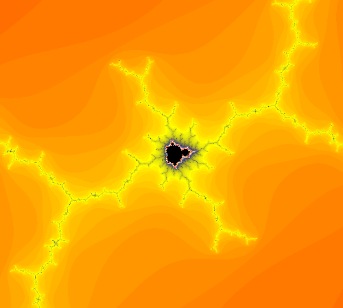
In this way we can exacly connect the Mandelbrot set on the real line to the logistic bifurcation map. One immediately interesting corollary of this finding is the fact that we can see our third-degree minibrot hiding amongst the bifurcation map all along. Despite the fact that the map looks extremely chaotic after the constant $r\approx 3.56995$, there are still some regions of stability. In fact, if we look at the region close to $3.84$ corresponds to our largest minibrot with cycle 3 and if we look at the region close to $3.63$ we get another region of stability with cycle 6, corresponding to another one of our minibrots.
3-cycle at $r=3.84$, $c=-1.76$ 6-cycle at $r=3.63$, $c=-1.48$

We can again see that as we go further right on the logistic diagram or further left of the Mandelbrot needle, we always get the period doubling effect sometimes called the "period-doubling cascade." One of the first questions I had after realizing how many of these minibrot sets were on the real line was: "Is any part of the logistic diagram chaotic at all? Or is it just very small regions of very large cycles like 17, 390, and 81054 but we just can't tell?" It turns out, as discussed in this blog that the answer actually is no! There really is true chaos along the Mandelbrot needle/ logistic bifurcation diagram in the sense that there is a positive measure region of chaos!
Okay, that was my last cool thing about the Mandelbrot set and hopefully you enjoyed this discussion post. Please feel free to explore all of this even further! I provide some of the resources I used for visualization in the final section of appendices. I will also include some extra reading references and the next section is a quick discussion of the theoretical gaps we had along the way and some directions to actually prove/ resolve these untouched facts.
Closing Some Gaps (Complex Analysis - Iterating Rational Functions)
Fatou's 1919 Theorem
We want to know how to show the fact that for a rational map, a solution to $f'(z)=0$ must fall in to the attracting cycle if there is one at all. An excellent write up of this fact can be found in https://link.springer.com/content/pdf/10.1007%2F978-1-4612-4364-9_3.pdf on pages 58-60 for Theorem 2.1 and Theorem 2.2.
Attractive Cycles will attract Zero
Throughout practically all of our calculations in this blog, we show the existence of an attractive cycle for certain parameter values $c$. A priori, there is no reason that we should expect the existence of any attractive cycles across the entire complex planes implies that the seed of zero (where we always start for the Mandelbrot set) will correspond to falling into exactly the attractive cycle which was found. Well, if we look above very quickly we can see that for the Mandelbrot rational map $f(z) = z^2+c$ we have $f'(z) = 2z$ which has unique critical point $0$. Hence, by Fatou's Theorem again, we can see that it is sufficient to check for the seed $z=0$.
Superattractive Points Describe Basins
In our later section, we looked into how each of the superattractive cycles should correspond to the centers of the basins of the attractive cyclic regions. We know that clearly by the continuity of the fixed point polynomials, that a superattracting seed will correspond to a region of attracting cycles, but the question is whether there can exist a region with small gradient norm (attracting derivative), which does not have any super-attracting cycles nearby in parameter space. For this I must admit that I could not find a proof, but it seems likely to be the case that there are no more attracting cycle basins than there are superattracting cycles points.
Additional Resources
Graphical Tools
Here is the main tool I was using for visualization of the Mandelbrot set http://www.jakebakermaths.org.uk/maths/mandelbrot/canvasmandelbrotv12bak7512.html. Thankfully, this tool was able to give a lot more control compared to other online Mandelbrot visualization tools which meant I didn't need to build my own in order to write this blog post.
Some of the other tools I was using were: geogebra, desmos, and mathematica.
It is obligatory that I provide my favorite Mandelbrot zoom as a part of this post.
Theory References
- https://people.ucsc.edu/~fmonard/Sp17_Math207/lecture18.pdf
- https://link.springer.com/content/pdf/10.1007%2F978-1-4612-4364-9_3.pdf
- https://www.matem.unam.mx/~omar/no-wandering-domains.html
Other References
- https://en.wikipedia.org/wiki/Logistic_map
- https://upload.wikimedia.org/wikipedia/commons/7/7d/LogisticMap_BifurcationDiagram.png
- https://nexus316.wordpress.com/fractals/real_chaos/